Now that I have a more ideal NavBot, with its thinner wheels and higher resolution encoders, my focus has turned in earnest to better understanding and dealing with odometry related errors typical for small two-wheeled robots with differential steering.

I have already touched briefly on systematic and non-systematic errors in a previous post and I plan to go into much more detail in a future one, but for now I just want to document my success with using a very neat technique to measure and correct for three of the most common systematic errors.

But first a little background on the errors themselves.

It’s the Wheels

All three of these errors are due to the real world characteristics of a robot’s wheels.

Our odometry calculations are very simplistic and make the following incorrect assumptions about the wheels:

1. That they are perfect discs and do not deform under load
2. That they have the exact same diameters
3. That they have no thickness

You can see this when we look at the way the Navigator calculates movement and changes in orientation:

The three equations that make use of our incorrect assumptions are:

Sl = D π Tl / Tt

Sr = D π Tr / Tt

θ = (Sl – Sr)/b

The calculations for Sl and Sr assume the wheels are perfect discs and have the exact same diameters (D). The calculation for heading change (θ) assumes we know what the true the wheelbase (b) is, which we can only know for sure if the wheels have no thickness.

Of course, in reality the wheels will have some thickness and while we can nominally measure b as the distance between the centers of where the tires contact the ground, the true wheelbase will most likely differ.

Similarly for wheel diameters, we can nominally measure them but in practice the wheels will deform under load, i.e. tires will compress by some amount, and so their effective diameters will differ too.

Wheelbase Error

Having an incorrect wheelbase value has the effect that we will either over-reporting or under-reporting changes in orientation. If we tell the robot to turn 90° it will either turn more than ninety or less than ninety. The difference from ninety is the wheelbase error and it is a systematic one, meaning it is proportional and consistent.

The error is directly proportional to the effective wheelbase divided by the nominal wheelbase :

Eb = actual wheelbase / nominal wheelbase

so we can correct for this error by multiplying the nominal wheelbase (bn) by the error factor to give us the effective wheelbase (be):

be = Eb * bn

Simple.

Now our heading calculation can factor in this correction:

θ = (Sl – Sr)/(Eb *bn)

Wheel Errors

Having incorrect wheel diameters creates two other types of error.

The first, and simplest, is a scaling error due to the wheels having an average diameter (Da) that is smaller, or larger, than our measured nominal diameter (Dn).

This error results in the distance (S) being over or under reported. We can quantify this error as the ratio of actual distance traveled to the distance reported, thus:

Es = Actual distance / Reported distance

Again we can adjust the nominal diameter (Dn) to the average one (Da):

Da = Es * Dn

And our distance calculations now become:

Sl = Es * Dn * π * Tl / Tt

Sr = Es * Dn * π * Tr / Tt

The last type of error is much tricker to deal with. If there is a difference in effective wheel diameters between the wheels, which will mostly certainly be the case, then even though we turn both wheels the same amount, one wheel will travel further than the other. The robot will think it is traveling in a straight line, i.e. Sl and Sr are the same, but in reality it is traveling in a slight curve.

Again this is another systematic error and is directly proportional to the relative sizes of the wheels:

Ed = Right wheel’s effective diameter / Left wheel’s effective diameter

Ed = Dr / Dl

Correcting for this error is a little more involved than the others as we want to adjust the left and right distances (Sl and Sr) but we do not want to alter the Es correction we’ve already added so the correction for right and left wheels becomes:

Cr = 2 / ( 1/Ed + 1)

Cl = 2 / ( Ed + 1)

So, finally, we have all of our new error adjusted calculations:

Sl = Cl * Es * Dn * π * Tl / Tt

Sr = Cr * Es * Dn * π * Tr / Tt

θ = (Sl – Sr)/(Eb *bn)

How to measure Es, Eb, and Ed?

So now that we know how to correct for the errors, how do we measure them?

Es is trivial to figure out. Make the robot travel in a straight line for a specific distance, measure the actually distance it travels and then divide the measured distance by the specified distance. Done.

Measuring Eb and Ed is a little more involved. Up till now I’ve used trial and error with mixed results.

For Eb (wheelbase error) I would make the robot spin for a certain number of revolutions and slowly adjust the value of Eb till the robot finished up at the correct orientation. The more revolutions performed the more accurate I could get the adjustment.

For Ed (wheel errors) I would make the robot travel in a straight line and adjust Ed till I got it to actually travel in a straight line.

While I got reasonable results it was not optimal and could be very time consuming. My biggest problem was not knowing if the bot was truly traveling in a straight line as I could only eyeball things and even using a laser pointer was of limited benefit.

However, there is a well known method for measuring Ed and Eb called The UMBmark Test. It is super easy to do, gives great results and doesn’t require laser pointers or anything like that. You just need a ruler and some paper.

The UMBmark Procedure

This procedure for determining Eb and Ed was developed by Johann Borenstein and Liqiang Feng around 1995 in the University of Michigan’s Advanced Technologies Lab. You can read about it in more detail in this paper from 1996 called “Measurement and Correction of Systematic Odometry Errors in Mobile Robots”.

I’ll provide a brief overview of how it works but you should refer to the paper to get an in-depth understanding of the math and principles.

First thing to note is that the procedure assumes that the dominant errors are due to wheelbase and wheel diameters only and all other error sources are either minimal or have been removed.

For example, it would impractical to use this method on rough uneven terrain or on surfaces that have traction issues. In fact, for my tests I used a 4×6 foot the granite countertop which happens to be the smoothest surface in my house. You would also need to make sure that you first fix any problems with the hardware and/or software. For example, verify that encoders are working and PID controllers are tuned properly. Your bot might not be traveling in straight line because the wheels are not turning at the same velocity.

You will also need to first measure Es and correct for it before proceeding.

The gist of the actual procedure is to have the robot move forward in a straight line for distance L, stop, turn 90° and repeat three more times so that it moves about a square of sides L, stopping and turning, in-place, at each corner and finally finishing back where it started. The test is performed in both clockwise and counter clockwise directions and we’ll see why in a while.

The paper classifies wheelbase error as Type A and errors related to differences in wheel diameters as Type B.

If your robot had only Type A errors then it would travel in perfectly straight lines but at the corners it would turn some amount more or less than 90° depending on the size of the error. They label this difference in angle as α.

Say we had a robot where α was -3°, i.e. it only turned 87° rather than 90°, then as it moved about the square it would finish at some (x, y) offset from the start position (0, 0).

Similarly if we went in a counter clockwise direction we would get the same displacement except that it would be mirrored about the y axis.

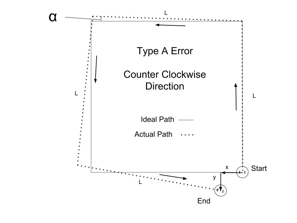
You can see from the geometry that it would easy to calculate α knowing x, y and L. That is the beauty of the UMBmark method. We don’t have to measure angles directly (which is hard to do accurately). Instead we just need to measure offset of the end position from the start position which is easy to do accurately.

Once we know α then calculating Eb is trivial:

Eb = 90° / ( 90° – α)

On the other hand, if our robot had only Type B errors it would make perfect 90° turns but move in an arc rather than a straight line. At the end of each leg of the square the robot will have drifted off course and changed it’s heading by some amount, depending on severity of the Type B error.

This change in the heading they label as angle β and it too will cause the robot to finish at some (x, y) offset from the starting position. Again, using geometry we can calculate β.

However, unlike Type A errors, Type B errors are not symmetrical. The same β error in the counter clockwise direction results a very different (x, y) offset from the start position.

This asymmetry is important as we shall see when we look at what can happen when both errors happen at the same time.

It is possible that Type A and B errors cancel each other out and give the impression that there is no error.

For example, say β is -3° and α is 3°. In the clockwise direction the over turning by 3 degrees happens to correct the 3 degree change in orientation caused by the Type B error as we can see from this diagram.

The robot will finish correctly at the start position. However, if we do the test in the counter clockwise direction the errors now compound one another and we can clearly see there is a problem.

This is partially why the UMBmark procedure uses both clockwise and counter clockwise measurements to accurately calculate α and β. Of course the main reason is that the asymmetry in geometry provides the two simultaneous equations needed to solve for both α and β. Really neat. Refer to the paper to see the math in action.

So the actual steps of the procedure are:

1. Mark the start position of the robot
2. Make it travel clockwise about a square of size L.
3. Mark the end position and measure the x and y difference from the start position.
4. Repeat this four more times in the clockwise direction.
5. Average the 5 results to get a COG x and y
6. Then repeat the above steps in the counter clockwise direction
7. Apply the COG x and y values for the clockwise and counter clockwise direction to the UMBmark formulas to obtain Eb and Ed

The reason for performing the tests 5 times in both directions is to minimize the effect of non-systematic errors. Non-systematic errors are relatively random in nature so averaging multiple runs should cancel out their effect somewhat.

The averaging, in effect, gives us a kind of “center of gravity” (COG) for the systematic errors.

What size should the square (L) be? That will most likely be dictated by how much space you have do your tests in. In my case the max size I could do was 800 mm. Obviously the larger the square then the greater the effect of the Type B errors.

Once we have the COG values for x and y in both CW and CCW directions we can use the following formulas to calculate Eb and Ed.

Using x values we can calculate α and β (in radians):

α = (Xccw – Xcw)/-4L

β = -(Xcw + Xccw)/-4L

Or using y values:

α = (Ycw + Yccw)/-4L

β = (Ycw – Yccw)/-4L

[Note that the above formulas differ from the paper I referenced at the start. This is due to the fact that NavBot uses a different coordinate system, which I explain in the next section.]

With β we can calculate Ed:

R = (L/2) / Sin(β/2)

Ed = (R + b/2) / (R – b/2)

Converting α into degrees we can calculate Eb:

Eb = 90° / ( 90° – α)

Using UMBmark For NavBot

So after all that theory how does it stack up in practice?

The first step was to modify Navigator to use the Es, Ed and Eb scalers.

Here are the pertinent code changes:

void SetWheelRLScaler( float Ed)
{
  m_wheel_rl_scaler = Ed;
}

void SetWheelbaseScaler( float Eb )
{
  m_wheelbase_scaler = Eb;
}

void SetDistanceScaler( float Es)
{
  m_dist_scaler = Es;
}

//----------------------------------------
//
//----------------------------------------

void Navigator::Reset( nvTime now )
{
  :
  :
  // calc odomerty terms
  m_effective_wheelbase = m_nominal_wheelbase*m_wheelbase_scaler;
  m_effective_wheel_diam = m_nominal_wheel_diam*m_dist_scaler;
  float dist_per_tick = m_effective_wheel_diam*M_PI/m_ticks_per_rev;
  float invE = 1.0f/m_wheel_rl_scaler;
  m_rticks_to_dist = dist_per_tick*(2.0f/(invE+1.0f));
  m_lticks_to_dist = dist_per_tick*(2.0f/(m_wheel_rl_scaler+1.0f));
}

//----------------------------------------
//
//----------------------------------------

bool Navigator::UpdateTicks( .... )
{
  :
  :
  nvDistance sr = ((nvDistance)m_rticks)*m_rticks_to_dist;
  nvDistance sl = ((nvDistance)m_lticks)*m_lticks_to_dist;
  nvDistance s = (sr + sl)*0.5f;

  // calc and update change in heading
  nvRadians theta = (sl - sr)/m_effective_wheelbase;
  m_heading = nvClipRadians( m_heading + theta);
  :
  :
  :
  // update pose
  m_pose.heading = nvRadToDeg(m_heading);
  m_pose.position.x += s*sin(m_heading);
  m_pose.position.y += s*cos(m_heading);
  :
  :
}

I then had to modify to the BlackBot.h code to set the initial error scalers, as well as the nominal values for wheelbase and wheel diameter:

// Navigator defines
#define WHEELBASE           nvMM(78.0)
#define WHEEL_DIAMETER      nvMM(32.0)
#define TICKS_PER_REV       909
#define WHEEL_RL_SCALER     1.0f   // Ed
#define WHEELBASE_SCALER    1.0f   // Eb
#define DISTANCE_SCALER     1.0f   // Es

The full code is on GitHub: NavBot Version 1

I also created a google spreadsheet to record and graph the results of the test, as well as calculate the E values:

I’ll explain how the worksheet is used as we go along.

You can access a view-only version of the it here: UMBmark Worksheet V1

Finding Es

The top left section of the worksheet is used to calculate Es which is the very first test that needs to be performed before we move on to UMBmark proper.

For this series of tests I configure the NavBot to travel in a straight line for 2 meters using the CALIBRATE_MOVE and CAL_DISTANCE defines at the top of NavBot_v1.ino. I also enabled TARGET_INFO so that the bot outputs its precise position at each waypoint via bluetooth.

//----------------------------------------
// Config Logic
//----------------------------------------
 :
 :
#define CFG_CALIBRATE_MOVE 1  // straight line movement
 :
#define CAL_DISTANCE   2  // meters to move for CALIBRATE_MOVE
 :
//----------------------------------------
// Serial output config
//----------------------------------------
 :
#define TARGET_INFO   1   // print nav data at way points
 :

In this configuration I let the bot travel the 2 meters and measure the actual distance it travelled, as well as recording the TARGET_INFO output for the y coordinate which gives us the exact distance the bot thought it travelled. The difference between these two number is the scaling error.

I performed this test three times and entered the values into the “Run 1”, “Run 2” and “Run 3” boxes. The values are averaged out to give the Es, in the yellow box, for this first phase.

I then set DISTANCE_SCALER to the new phase 1 Es value and ran the tests again but this time inputing the results into the phase 2 boxes to obtain a more accurate value for Es in phase 2’s yellow box. This new value already factors in Es from phase 1 so you can input the value directly to the bot and run the test again for phase 3.

At that point the difference between the measured distance and reported distance should be very small indeed. You can see from my results that the final average error was under a millimeter after the phase 2 correction, which is about as accurate as I can measure.

Doing the Square Tests

To setup the robot to do the square test I enabled SQUARE_TEST in the config settings at the top of NavBot_v1.ino and set SQUARE_SIZE to 800:

//----------------------------------------
// Config Logic
//----------------------------------------

#define CFG_TEST_ENCODERS     0     // print encoder ticks
#define CFG_TEST_MOTORS       0     // verify motor wiring
#define CFG_SQUARE_TEST       1
#define CFG_CALIBRATE_MOVE    0     // straight line movement
#define CFG_CALIBRATE_TURNS   0     // turning only test
 :
 :
#define SQUARE_SIZE       800   // size of square test in mm

Then set testPath to cwSquare for the clockwise tests and to ccwSquare for the counter clockwise tests:

int16_t *testPath = cwSquare;

Once I had the bot configured I used a very smooth granite counter top in my kitchen to run the tests on:

A ruler and taped down sheets of graph paper was all that was needed to mark and measure the start and end positions of each run.

Note that whatever method you decide to employ to mark the robot’s position be mindful that it is not affected by rotation of the bot, i.e. do not mark just one point on the perimeter of the robot as that will give you erroneous results.

The results of all the runs – 5 clockwise and 5 counter clockwise – where entered into the worksheet.

Along with the size of the square, which in my case is 800 mm and the wheelbase which is 78 mm.

BTW, all my measurements are in mm. I omitted specifying actual units in the spreadsheet so that people could use inches if they so desired.

On the right you can see where it calculates Ed and Eb for both x and y and then averages them.

Another important point to note if you decided to use the worksheet for your own tests, is that the calculations for Eb and Ed are based on the coordinate system used by Navigator.

Navigator defaults to heading zero, i.e. North, which is in the direction of the positive y axis. If you use a different system then you might need to adapt the formulas accordingly.

A cool thing about spreadsheets is that we can make pretty graphs of the data. Here is the first run with Ed and Eb both set to 1.0:

The units are in mm.

I updated the robot with the newly calculated values for Eb and Ed:

// Navigator defines
#define WHEELBASE           nvMM(78.0)
#define WHEEL_DIAMETER      nvMM(32.0)
#define TICKS_PER_REV       909
#define WHEEL_RL_SCALER     1.002463028f   // Ed
#define WHEELBASE_SCALER    0.9918532967f  // Eb
#define DISTANCE_SCALER     1.004642139f   // Es

Ran the tests again and got another pretty graph:

You can see that the error has been greatly reduced – by about 6 fold.

We can also apply the newly calculate values from the second run to get even better accuracy. In this case we have to multiple the values from the first run with the second:

/// Navigator defines
#define WHEELBASE           nvMM(78.0)
#define WHEEL_DIAMETER      nvMM(32.0)
#define TICKS_PER_REV       909
#define WHEEL_RL_SCALER     (1.002463028f*1.000276208f)
#define WHEELBASE_SCALER    (0.9918532967f*0.9990412995f)
#define DISTANCE_SCALER     1.004642139f

While the graphs do look cool, and scientific, they did have a practical purpose. I was able to visually verify I had entered the data in correctly by comparing the spreadsheet graphs to my physical paper plots.

All in all I’m very pleased with how things turned out. NavBot is starting to shape up nicely.

I plan to follow up on another paper – Accurate calibration of kinematic parameters for two wheel differential mobile robots by Kooktae Lee et al – where the authors propose a modified UMBmark test that addresses the fact that Type A and Type B errors are not independent of each other; an assumption that the original method makes.